Matrizen: Unterschied zwischen den Versionen

Rechenregeln

Merke

Bei der Addition von Matrizen, werden die gleichen Komponenten miteinander addiert. Sei die Matrix $ A= \begin{pmatrix} a_{11} & a_{12} & \dots & a_{1n} \\ a_{21} & a_{22} &\dots & a_{2n} \\ \vdots & \vdots &\ddots & \vdots \\ a_{m1} & a_{m2} & \dots & a_{mn} \end{pmatrix} $ und die Matrix $ B= \begin{pmatrix} b_{11} & b_{12} & \dots & b_{1n} \\ b_{21} & b_{22} &\dots & b_{2n} \\ \vdots & \vdots &\ddots & \vdots \\ b_{m1} & b_{m2} & \dots & b_{mn} \end{pmatrix} $ dann ist $A +B = \begin{pmatrix} a_{11} + b_{11} & a_{12}+ b_{12} + & \dots +& a_{1n} + b_{1n} \\ a_{21} + b_{21} & a_{22} + b_{22} + &\dots +& a_{1n}+ b_{2n} \\ \vdots & \vdots &\ddots & \vdots \\ a_{m1}+ b_{m1} &a_{m2} + b_{m2} & + \dots +& a_{mn} + b_{mn} \end{pmatrix} $ Bei der Addition müssen beide Matrizen dieselbe Dimension haben, das heißt dieselbe Anzahl von Zeilen und Spalten.

Bei der $2\times 2$ Matrix schaut das wie folgt aus

$ A= \begin{pmatrix} a_{11} & a_{12} \\ a_{21} & a_{22} \\ \end{pmatrix} $

$ B= \begin{pmatrix} b_{11} & b_{12} \\ b_{21} & b_{22} \\ \end{pmatrix} $

dann ist $ \qquad \qquad \qquad A+ B =\begin{pmatrix}a_{11} & a_{12} \\ a_{21} & a_{22} \end{pmatrix} + \begin{pmatrix} b_{11} & b_{12} \\ b_{21} & b_{22} \end{pmatrix} = \begin{pmatrix} a_{11} + b_{11} & a_{12} + b_{12} \\ a_{21} + b_{21} & a_{22} + b_{22} \\ \end{pmatrix}$

Addiere die beiden Matrizen und füge die Zahlen der Lösungsmatrix in die Zellen ein, dann klicke auf überprüfen.

Subtrahiere die beiden Matrizen und füge die Zahlen der Lösungsmatrix in die Zellen ein, dann klicke auf überprüfen.

Merke

Bei der Multiplikation mit einem Skalar $k$ (einer reellen Zahl), wird jede Komponente einzeln mit dem Skalar multipliziert. $ k \cdot A= \begin{pmatrix} k \cdot a_{11} & k \cdot a_{12} & \dots & k \cdot a_{1n} \\ k \cdot a_{21} & k \cdot a_{22} & \dots & k \cdot a_{2n} \\ \vdots & \vdots & \ddots & \vdots \\ k \cdot a_{m1} &k \cdot a_{m2} & \dots & k \cdot a_{mn} \\ \end{pmatrix} $

Multipliziere die Matrix mit dem Skalar und füge die Zahlen der Lösungsmatrix in die Zellen ein, dann klicke auf überprüfen.

Definition

Transponierte Matrix Bei einer transponierten Matrix werden die Zeilen und Spalten miteinander vertauscht. Sei $A$ die ursprüngliche Matrix und $A^T$ die transponierte Matrix: $A= \begin{pmatrix} a_{11} & a_{12} &a_{13} \\ a_{21} & a_{22} & a_{23} \\ a_{31} &a_{32} & a_{33} \\ \end{pmatrix} $ dann ist $A^T= \begin{pmatrix} a_{11} & a_{21} &a_{31} \\ a_{12} & a_{22} & a_{32} \\ a_{13} &a_{23} & a_{33} \\ \end{pmatrix} $

Definition

Matrizenmultiplikation Zwei Matrizen werden nach der Regel: Zeile mal Spalte multipliziert. Die Matrizenmultiplikation ist nicht kommutativ, das heißt: $A\cdot B \neq B \cdot A$. Um $A \cdot B =C$ zu erhalten muss die Anzahl der Spalten von $A$ die selbe sein wie die Anzahl der Zeilen von $B$. Also wenn $A$ eine $m \times n$ Matrix ist und $B$ eine $n \times p$ Matrix, so sind $m$ und $p$ beliebig und $n$ muss bei $A$ und $B$ dieselbe Zahl sein. Außerdem ist dann $C$ eine $m \times p$ Matrix, sie hat also dieselbe Anzahl der Zeilen wie die Matrix $A$ und dieselbe Spaltenanzahl wie die Matrix $B$.

Sei die Matrix $A$ zum Beispiel eine $2 \times 3$ Matrix und $B$ eine $3 \times 4$ Matrix. Dann ist die Matrix $A \cdot B = C$ eine $2 \times 4$ Matrix.

Wie erhält man nun die einzelnen Koeffizienten der Matrix $C$?

\url{https://www.youtube.com/watch?v=iLgfkgscafQ}

Die Durchführung der Matrizenmultiplikation kann mit Hilfe der Falk'schen Anordnung erfolgen:

$ \begin{pmatrix} b_{11} & b_{12} & \dots & b_{1q} \\ b_{21} & b_{22} & \dots & b_{2q} \\ \vdots & \vdots & \ddots & \vdots \\ b_{p1} & b_{p2} & \dots & b_{pq} \\ \end{pmatrix} $ $ \begin{pmatrix} a_{11} & a_{12} & \dots & a_{1p} \\a_{21} & a_{22} & \dots & a_{2p} \\ \vdots & \vdots & \ddots & \vdots \\ a_{n1} & a_{n2} & \dots & a_{np}\\ \end{pmatrix} $ $ \begin{pmatrix} c_{11} & c_{12} & \dots & c_{1q}\\ c_{21} & c_{22} & \dots & c_{2q} \\ \vdots & \vdots & \ddots & \vdots \\ c_{n1} & c_{n2} & \dots & c_{nq} \end{pmatrix} $ Es werden die Spalten von $B$ über die Zeilen von $A$ gelegt, die Komponenten paarweise multipliziert und dann die Ergebnisse addiert.

Wobei $$c_{11} = a_{11} \cdot b_{11}+ a_{12} \cdot b_{21} + \dots + a_{1p} \cdot b_{p1} \\ c_{12} = a_{11} \cdot b_{12} + a_{12} \cdot b_{22} + \dots + a_{1p} \cdot b_{p2} \\ c_{1q} = a_{11} \cdot b_{1q} + a_{12} \cdot b_{2q} + \dots + a_{1p} \cdot b_{pq} \\ \vdots \\ c_{21} = a_{21} \cdot b_{11} + a_{22} \cdot b_{21} + \dots + a_{2p} \cdot b_{p1}\\ \vdots \\ c_{nq} = a_{n1} \cdot b_{1q} + a_{n2} \cdot b_{2q}+ \dots + a_{np} \cdot b_{pq}$$

Konkret heißt das an einem Beispiel:

	$ \begin{pmatrix} 8 &1 & 3 \\9 & 0 & 5 \\ \end{pmatrix} $
$ \begin{pmatrix} 2 & 5 \\4 & 7 \\ \end{pmatrix} $	$ \begin{pmatrix} c_{11} & c_{12} & c_{13}\\ c_{21} & c_{22} & c_{23} \\ \end{pmatrix} $

Wobei $$c_{11} = 2 \cdot 8 + 5 \cdot 9 = 61\\ c_{12} = 2 \cdot 1 + 5 \cdot 0 =2\\ c_{13} = 2 \cdot 3 + 5 \cdot 5 =31\\ c_{21} = 4 \cdot 8 + 7 \cdot 9 =95\\ c_{22} = 4 \cdot 1 + 7 \cdot 0 =4\\ c_{23}= 4 \cdot 3 + 7 \cdot 5 =47$$ Also $$\begin{pmatrix} 2 & 5 \\ 4 & 7 \\ \end{pmatrix} \cdot \begin{pmatrix} 8 &1 & 3 \\ 9 & 0 & 5 \\ \end{pmatrix} = \begin{pmatrix} 61 & 2 & 31\\ 95 & 4 & 47 \\ \end{pmatrix} $$

Multipliziere die beiden Matrizen und füge die Zahlen der Lösungsmatrix in die Zellen ein, dann klicke auf überprüfen.

Gozinto-Graphen

Gonzinto-Graphen dienen der Veranschaulichung der Zusammenhänge zwischen Roh-, Zwischen- und Endprodukten. Die Knoten stellen dabei die Teile dar und die Pfeile oder auch gerichtete Kanten die Mengenbeziehungen.

In der Abbildung des Gozintographen wird der Zusammenhang zwischen den Rohstoffen $R_1 , R_2$ und $R_3$ mit den Zwischenprodukten $Z_1, Z_2, Z_3$ und den Endprodukten $E_1, E_2$ dargestellt.

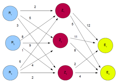
In einer Tabelle kann der Zusammenhang wie folgt aufgelistet werden:

	$Z_1$	$Z_2$	$Z_3$
$R_1$	2	5	3
$R_2$	8	9	1
$R_3$	6	4	2

	$E_1$	$E_2$
$Z_1$	12	5
$Z_2$	11	8
$Z_3$	2	4

Die Tabelle kann aber ebenso in Matrixform umgeschrieben werden, wobei die Matrix $RZ$ den Zusammenhang der Rohstoffe mit den Zwischenprodukten und $ZE$ den der Zwischenprodukte mit den Endprodukten beschreibt.

$$ RZ= \begin{pmatrix} 2 & 5 & 3 \\8 & 9 &1 \\ 6&4&2\\ \end{pmatrix} $$ $$ ZE=\begin{pmatrix} 12 & 5 \\ 11 & 8 \\ 2&4\\ \end{pmatrix} $$

Um eine Matrix zu erhalten, welche den Rohstoffbedarf für die Endprodukte beschreibt wird die Matrix $RZ$ mit der Matrix $ZE$ multipliziert. In unserem Beispiel ergibt das

\begin{equation*} RE= RZ \cdot ZE= \begin{pmatrix} 24 +55+ 6 & 10 +40+ 12\\ 96 +99 +2 & 40+ 72+ 4\\ 72 +44+ 4 & 30+ 32+ 8\\ \end{pmatrix} = \begin{pmatrix} 85 &62\\ 197 & 116\\ 120 & 70\\ \end{pmatrix}. \end{equation*}

Die Matrizen $RZ$, $ZE$ und $RE$ werden auch Produktionsmatrix genannt. Der Produktions-, Output- oder Nachfragevektor gibt an wie viel der Endprodukte produziert werden sollen. Der Bedarfsvektor gibt den Gesamtbedarf an Einzelteilen an für einen vorgesehenen Produktionsvektor. Also durch den Bedarfsvektor kann der Bedarf an Rohstoffen berechnet werden.

Im Preisvektor befinden sich die Preise für die einzelnen Rohstoffe. Der Inputvekor beschreibt die benötigten Rohstoffe.

Input-Output-Matrix: Leontief-Modell

Eine Input-Output-Tabelle für die Firmen A, B und C, mit $x_i=\sum_{k=1}^{3} x_{ik} y_i$, wobei $i=j$ den Eigenbedarf einer Firma beschreibt, wird in der folgenden Tabelle aufgezeigt.

Input / Output	A	B	C	Markt / Konsum	Gesamtproduktion
A	$x_{11}$	$x_{12}$	$x_{13}$	$y_{1}$	$x_{1}$
B	$x_{21}$	$x_{22}$	$x_{23}$	$y_{2}$	$x_{2}$
C	$x_{31}$	$x_{32}$	$x_{33}$	$y_{3}$	$x_{3}$

In einem Gozinto-Graphen kann dies, wie rechts unten zu sehen ist, dargestellt werden:

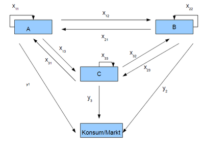
Die Produktionsmatrix $P$ sieht daher folgendermaßen aus:

$P=\begin{pmatrix} x_{11} & x_{12} & x_{13} \\ x_{21} & x_{22} & x_{23} \\x_{31} & x_{32} & x_{33}\\ \end{pmatrix}.$

Um die Input-Output-Matrix zu erhalten die erste Spalte durch den Wert der Gesamtproduktion der ersten Zeile geteilt werden, die zweite Spalte durch den der zweiten Zeile und die dritte Spalte durch den der dritten Zeile, das heißt die Koeffizienten der Input-Output-Matrix ergeben sich als $a_{ij}= \frac{x_{ij}}{x_j}$

Die Input-Output-Matrix ergibt sich dann zu: $M=\begin{pmatrix} \frac{x_{11}}{x_1} & \frac{x_{12}}{x_2} & \frac{x_{13}}{x_3} \\ \frac{x_{21}}{x_1} & \frac{x_{22}}{x_2} & \frac{x_{23}}{x_3} \\ \frac{x_{31}}{x_1} & \frac{x_{32}}{x_2} & \frac{x_{33}}{x_3}\\ \end{pmatrix}.$

Dieser und die folgenden Abschnitte sind nur für HTL-SchhülerInnen relevant.

Saklierungsmatrix

Um einen Vektor zu stauchen oder zu strecken, wird er mit einem Faktor multipliziert.

\begin{align*} x'&=x \cdot s_x\\ y'&=y\cdot s_y \\ z' &= z \cdot s_z \end{align*} In Matrixform kann er mit der Skalierungsmatrix multipliziert werden.

$$U=\begin{pmatrix}s_x & 0 & 0\\ 0 & s_y & 0 \\ 0& 0 &s_z \\ \end{pmatrix} $$ Dabei gibt $s_x$ die Skalierung in x-Richtung, $s_y$ die Skalierung in y-Richtung und $s_z$ die Skalierung in z-Richtung an.

Drehung

Die Drehung ist ein Beispiel für die Anwendung und Motivation der Matrizenmultiplikation. In $\mathbb{R}^2$ und $\alpha \in [0, 2 \pi[$ wird die Drehung (gegen den Uhrzeigersinn) eines Vektors $v$ um den Winkel $\alpha $ durch die Multiplikation des Vektors mit der Drehmatrix $$R_{\alpha} \begin{pmatrix} \cos(\alpha) & -\sin(\alpha) \\\sin(\alpha) & \cos(\alpha) \\ \end{pmatrix} $$ erreicht: $v'=R_\alpha \cdot v$.

In $\mathbb{R}^3$ ergeben sich für die Drehungen um die

• x-Achse:

$$R_x(\alpha)=\begin{pmatrix}1&0 & 0\\ 0& \cos(\alpha) & -\sin(\alpha) \\ 0& \sin(\alpha) & \cos(\alpha) \\ \end{pmatrix} $$

• y-Achse:

$$R_y(\alpha)=\begin{pmatrix}\cos(\alpha) &0 & \sin(\alpha) \\ 0& 1 & 0 \\ - \sin(\alpha)& 0 & \cos(\alpha) \\ \end{pmatrix} $$

• z-Achse

$$R_z(\alpha)=\begin{pmatrix}\cos(\alpha) & -\sin(\alpha) & 0\\ \sin(\alpha) & \cos(\alpha) & 0 \\ 0& 0 & 1 \\ \end{pmatrix} $$

homogene Koordinaten

Homogene Koordinaten werden zum Beispiel verwendet wenn eine Verschiebung eines Vektors durchgeführt werden soll, also wenn eine nicht lineare Transformation stattfindet.

Euklidische Koordinaten in $\mathbb{R}^3$ werden wie folgt in homogenen Koordinaten umgeschrieben $$\begin{pmatrix} x\\ y\\ z \end{pmatrix} \mapsto \begin{bmatrix} x \\ y\\ z\\1 \end{bmatrix} .$$

Schiebung

Die Schiebung eines Vektors $\begin{pmatrix} x\\ y\\ \end{pmatrix}$ um den Vektor $\begin{pmatrix} t_x \\ t_y \\ \end{pmatrix}$ ist nicht linear und deshalb müssen die Koordinaten in homogenen Koordinaten geschrieben werden, damit man die Schiebung in Matrixform schreiben kann.

So erhält man für die Translation:

\begin{align*} x'&=x + t_z \\ y'&= y +t_y \\ \end{align*} $\Rightarrow$

\begin{equation*} \begin{pmatrix} x'\\ y' \\ 1\\ \end{pmatrix} =\begin{pmatrix} 1 &0&t_x\\ 0&1& t_y\\ 0&0&1\\ \end{pmatrix} \cdot\begin{pmatrix} x\\ y\\1\\ \end{pmatrix}. \end{equation*}

Im $\mathbb{R}^3$ ergibt sich für die Schiebung

\begin{equation*} T_3=\begin{pmatrix} 1&0 &0&t_x \\ 0& 1 &0&t_y \\ 0&0&1& t_z \\ 0&0&0&1 \end{pmatrix} \end{equation*}

Spiegelung

Die Spiegelung ist ein Sonderfall der Skalierung mit entweder $s_x=-1$, $s_y=-1$ oder $s_z=-1$, je nachdem um welche Achse gespiegelt werden soll, die anderen Skalierungsfaktoren sollen dabei den Wert $1$ annehmen.

Es ergeben sich also die verschiedenen Spiegelungsmatrizen, je nach Spiegelungsachse: im $\mathbb{R}^2$:

• um die x-Achse:

$S_x=\begin{pmatrix} 1&0 \\ 0& -1 \\ \end{pmatrix}$

• um die y-Achse:

$S_y=\begin{pmatrix}-1&0 \\ 0& 1 \\ \end{pmatrix}$

-im $\mathbb{R}^3$

• um die yz-Ebene:

\begin{equation*} S_{yz}= \begin{pmatrix} -1&0 &0\\0& 1 &0\\ 0&0&1 \end{pmatrix} \end{equation*}

• um die xz-Ebene:

\begin{equation*} S_{xz}= \begin{pmatrix} 1&0 &0\\0& -1 &0\\ 0&0&1 \end{pmatrix} \end{equation*}

• um die xy-Ebene:

\begin{equation*} S_{xy}= \begin{pmatrix} 1&0 &0\\0& 1 &0\\ 0&0&-1 \end{pmatrix} \end{equation*}

Spiegelung an einer Geraden

Die Spiegelung eines Punktes im $\mathbb{R}^2$ an einer Gerade $g: y=ax+b$ erfolgt in homogenen Koordinaten in den folgenden fünf Schritten:

1.) Das Koordinatensystem so verschieben, dass die Spiegelungsachse durch den Koordinatenursprung geht.

2.) Die Spiegelungsachse soll um den Winkel $\arctan(a)$ gedreht werden, so dass sie mit der x-Achse zusammenfällt.

3.) Spieglung an der x-Achse.

4.) In Ausgangsposition zurückdrehen, also Schritt 2) in die andere Richtung.

5.) Die Spiegelungsachse zurück schieben, also wie in Schritt 1), nur in die andere Richtung schieben.

Damit die Matrizen alle miteinander multipliziert werden können, müssen sie in den selben Koordinaten geschrieben werden, da eine Translation angewendet wird, sollten alle Matrizen in homogenen Koordinaten angeschrieben werden.

Für die jeweiligen Schritte gibt es eine passende Matrix, werden die fünf Matrizen miteinander multipliziert erhält man die Spiegelungsmatrix um die Gerade $g$, mit $arctan(a):=t$.

$$ \begin{pmatrix} 1 & 0 & 0\\ 0 & 1 & b \\ 0& 0 & 1 \\ \end{pmatrix} \cdot \begin{pmatrix} \cos\left(t\right) & -\sin\left(t\right) & 0\\ \sin\left(t\right) & \cos\left(t\right) & 0 \\ 0& 0 & 1 \\ \end{pmatrix} \cdot\begin{pmatrix} 1 & 0 & 0\\ 0 & -1 & 0 \\ 0& 0 & 1 \\ \end{pmatrix} \cdot \begin{pmatrix} \cos\left(-t\right) & -\sin\left(-t\right) & 0\\ \sin\left(-t\right) & \cos\left(-t\right) & 0 \\ 0& 0 & 1 \\ \end{pmatrix} \cdot \begin{pmatrix} 1 & 0 & 0\\ 0 & 1 & -b \\ 0& 0 & 1 \\ \end{pmatrix} $$

Matura-Aufgaben

$Bifie$ RGB-Farbmodell

$Bifie$ "Spiegelung an einer Geraden"

$Bifie$ "Farben (2)"

$Bifie$ " "KP1_16_C2_06

$Bifie$ "Teemischung"

$Bifie$ "Rohstoffbedarf"

$Bifie$ "Konfiserie"

$Bifie$ "Zweistufige Produktion"

$Bifie$ "Kosten und Gewinn"